mjhjmtu

special function defined piecewise by polynomials

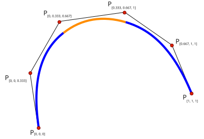
Single knots at 1/3 and 2/3 establish a spline of three cubic polynomials meeting with C² continuity. Triple knots at both ends of the interval ensure that the curve interpolates the end points

In mathematics, a spline is a function defined piecewise by polynomials. In interpolating problems, spline interpolation is often preferred to polynomial interpolation because it yields similar results, even when using low degree polynomials, while avoiding Runge's phenomenon for higher degrees.

In the computer science subfields of computer-aided design and computer graphics, the term spline more frequently refers to a piecewise polynomial parametric curve^{[citation needed]}. Splines are popular curves in these subfields because of the simplicity of their construction, their ease and accuracy of evaluation, and their capacity to approximate complex shapes through curve fitting and interactive curve design.^{[citation needed]}

The term spline comes from the flexible spline devices used by shipbuilders and draftsmen to draw smooth shapes.^[1] It also is an acronym for "Smooth Polynomial Lines Interpolating Numerical Estimates".

Introduction

The term "spline" is used to refer to a wide class of functions that are used in applications requiring data interpolation and/or smoothing. The data may be either one-dimensional or multi-dimensional. Spline functions for interpolation are normally determined as the minimizers of suitable measures of roughness (for example integral squared curvature) subject to the interpolation constraints. Smoothing splines may be viewed as generalizations of interpolation splines where the functions are determined to minimize a weighted combination of the average squared approximation error over observed data and the roughness measure. For a number of meaningful definitions of the roughness measure, the spline functions are found to be finite dimensional in nature, which is the primary reason for their utility in computations and representation. For the rest of this section, we focus entirely on one-dimensional, polynomial splines and use the term "spline" in this restricted sense.

Definition

The simplest spline is a piecewise polynomial function, with each polynomial having a single variable. The spline S takes values from an interval [a,b] and maps them to $mathbb R$ , the set of real numbers,

displaystyle S:[a,b]to mathbb R .

Since S is piecewise defined, choose k subintervals to partition [a,b]:

displaystyle [t_i,t_i+1]mbox , i=0,ldots ,k-1

displaystyle [a,b]=[t_0,t_1]cup [t_1,t_2]cup cdots cup [t_k-2,t_k-1]cup [t_k-1,t_k]

displaystyle a=t_0leq t_1leq cdots leq t_k-1leq t_k=b

Each of these subintervals is associated with a polynomial P_i,

displaystyle P_i:[t_i,t_i+1]to mathbb R

.

On the ith subinterval of [a,b], S is defined by P_i,

displaystyle S(t)=P_0(t)mbox , t_0leq t<t_1,

displaystyle S(t)=P_1(t)mbox , t_1leq t<t_2,

vdots

displaystyle S(t)=P_k-1(t)mbox , t_k-1leq tleq t_k.

The given k+1 points t_j (0 ≤ j ≤ k) are called knots. The vector
$displaystyle mathbf t =(t_0,dots ,t_k)$ is called a knot vector for the spline. If the knots are equidistantly distributed in the interval [a,b] we say the spline is uniform, otherwise we say it is non-uniform.

If the k polynomial pieces P_i each have degree at most n, then the spline is said to be of degree ≤ n (or of order ≤ n+1).

If for $displaystyle 1leq ileq k-1;:;Sin C^r_i$ in a neighborhood of the k-1 points t_i, then the spline is said to be
of smoothness (at least) $displaystyle C^r_i$ at t_i. That is, at t_i the two pieces P_i−1 and P_i share common derivative values from the derivative of order 0 (the function value) up through the derivative of order r_i (in other words, the two adjacent polynomial pieces connect with loss of smoothness of at most n - r_i).

A vector
$displaystyle mathbf r =(r_1,dots ,r_k-1)$ such that the spline has smoothness $displaystyle C^r_i$ at t_i for $displaystyle i=1,ldots ,k-1$ is called a smoothness vector for the spline.

Given a knot vector $displaystyle mathbf t$ , a degree n, and a smoothness vector $mathbf r$ for $displaystyle mathbf t$ , one can consider the set of all splines of degree $leq n$ having knot vector
$displaystyle mathbf t$ and smoothness vector $mathbf r$ . Equipped with the operation of adding two functions (pointwise addition) and taking real multiples of functions, this set becomes a real vector space. This spline space is commonly denoted by $displaystyle S_n^mathbf r (mathbf t )$ .

A knot t_i can be "deleted" by moving it to equal another knot t_i+1. The polynomial piece
P_i(t)
disappears, and the pieces
P_i−1(t) and P_i+1(t)
join with the sum of the continuity losses for
t_i and t_i+1.

That is,

displaystyle S(t)in C^n-j_i-j_i+1[t_i=t_i+1],

where

displaystyle j_i=n-r_i

This leads to a more general understanding of a knot vector. The continuity loss at any point can be considered to be the result of multiple knots located at that point, and a spline type can be completely characterized by its degree n and its extended knot vector

displaystyle (t_0,t_1,cdots ,t_1,t_2,cdots ,t_2,t_3,cdots ,t_k-2,t_k-1,cdots ,t_k-1,t_k)

where t_i is repeated j_i times
for $displaystyle i=1,dots ,k-1$ .

A parametric curve on the interval [a,b]

displaystyle G(t)=(X(t),Y(t))mbox , tin [a,b]

is a spline curve if both X and Y are spline functions
of the same degree with the same extended knot vectors on that interval.

Examples

Suppose the interval [a,b] is [0,3] and the subintervals are [0,1], [1,2], and [2,3]. Suppose the polynomial pieces are to be of degree 2, and the pieces on [0,1] and [1,2] must join in value and first derivative (at t=1) while the pieces on [1,2] and [2,3] join simply in value (at t = 2).

This would define a type of spline S(t) for which

displaystyle S(t)=P_0(t)=-1+4t-t^2mbox , 0leq t<1

displaystyle S(t)=P_1(t)=2tmbox , 1leq t<2

displaystyle S(t)=P_2(t)=2-t+t^2mbox , 2leq tleq 3

would be a member of that type, and also

displaystyle S(t)=P_0(t)=-2-2t^2mbox , 0leq t<1

displaystyle S(t)=P_1(t)=1-6t+t^2mbox , 1leq t<2

displaystyle S(t)=P_2(t)=-1+t-2t^2mbox , 2leq tleq 3

would be a member of that type.

(Note: while the polynomial piece 2t is not quadratic, the result is still called a quadratic spline. This demonstrates that the degree of a spline is the maximum degree of its polynomial parts.) The extended knot vector for this type of spline would be (0, 1, 2, 2, 3).

The simplest spline has degree 0. It is also called a step function. The next most simple spline has degree 1. It is also called a linear spline. A closed linear spline (i.e, the first knot and the last are the same) in the plane is just a polygon.

A common spline is the natural cubic spline of degree 3 with continuity C². The word "natural" means that the second derivatives of the spline polynomials are set equal to zero at the endpoints of the interval of interpolation

displaystyle S''(a),=S''(b)=0.

Algorithm for computing natural cubic splines

Cubic splines have polynomial pieces of the form $displaystyle P_i(x)=a_i+b_i(x-x_i)+c_i(x-x_i)^2+d_i(x-x_i)^3.$ Given $k+1$ coordinates $displaystyle (x_0,y_0),(x_1,y_1),dots ,(x_k,y_k),$ we find $k$ polynomials $displaystyle P_i(x),$ which satisfy for $displaystyle 1leq ileq k-1$ :

displaystyle P_0(x_0)=y_0quad

and

displaystyle quad P_i-1(x_i)=y_i=P_i(x_i),

displaystyle P'_i-1(x_i)=P'_i(x_i),

displaystyle P''_i-1(x_i)=P''_i(x_i),

displaystyle P''_0(x_0)=P''_k-1(x_k)=0.

One such polynomial $P_i$ is given by a 5-tuple $displaystyle (a,b,c,d,x)$ where $displaystyle a,b,c,$ and $d,$ correspond to the coefficients as used above and $x$ denotes the variable over the appropriate domain $[x_i,x_i+1]$ .

Computation of Natural Cubic Splines:

Input: a set of $k+1$ coordinates

Output: a spline as a set of polynomial pieces, each represented by a 5-tuple.

Create a new array a of size k + 1, and for $displaystyle i=0,ldots ,k$ set $displaystyle a_i=y_i$

Create new arrays b, d and μ each of size k

Create a new array h of size k and for $displaystyle i=0,ldots ,k-1$ set $displaystyle h_i=x_i+1-x_i$

Create a new array α of size k-1 and for $displaystyle i=1,ldots ,k-1$ set $displaystyle alpha _i=tfrac 3h_i(a_i+1-a_i)-tfrac 3h_i-1(a_i-a_i-1)$

Create new arrays c, l, and z each of size $k+1$ .

Set $displaystyle l_0=1,;mu _0=z_0=0$

For i=1,…,k−1displaystyle i=1,ldots ,k-1, $displaystyle i=1,ldots ,k-1,$
1. Set $displaystyle l_i=2(x_i+1-x_i-1)-h_i-1mu _i-1.$
2. Set $displaystyle mu _i=tfrac h_il_i.$
3. Set $displaystyle z_i=tfrac alpha _i-h_i-1z_i-1l_i.$

Set $displaystyle l_k=1;z_k=c_k=0.$

For j=k−1,k−2,…,0displaystyle j=k-1,k-2,ldots ,0 $displaystyle j=k-1,k-2,ldots ,0$
1. Set $displaystyle c_j=z_j-mu _jc_j+1$
2. Set $displaystyle b_j=tfrac a_j+1-a_jh_j-tfrac h_j(c_j+1+2c_j)3$
3. Set $displaystyle d_j=tfrac c_j+1-c_j3h_j.$

Create the spline as a new set of polynomials and call it output_set. Populate it with k 5-tuples for the polynomials P.

For i=0,…,k−1displaystyle i=0,ldots ,k-1 $displaystyle i=0,ldots ,k-1$
1. Set P_i,a = a_i
2. Set P_i,b = b_i
3. Set P_i,c = c_i
4. Set P_i,d = d_i
5. Set P_i,x = x_i

Output output_set

Continuity levels

If sampled data from a function or a physical object are available, spline interpolation is an approach to creating a spline that approximates those data.

Natural continuity

The classical spline type of degree n used in numerical analysis has continuity

displaystyle S(t)in mathrm C ^n-1[a,b],,

which means that every two adjacent polynomial pieces meet in their value and first n - 1 derivatives at each knot. The mathematical spline that most closely models the flat spline is a cubic (n = 3), twice continuously differentiable (C²), natural spline, which is a spline of this classical type with additional conditions imposed at endpoints a and b.

Reduced continuity

Another type of spline that is much used in graphics, for example in drawing programs such as Adobe Illustrator from Adobe Systems, has pieces that are cubic but has continuity only at most

displaystyle S(t)in mathrm C ^1[a,b].

This spline type is also used in PostScript as well as in the definition of some computer typographic fonts.

Many computer-aided design systems that are designed for high-end graphics and animation use extended knot vectors, for example Maya from Alias. Computer-aided design systems often use an extended concept of a spline known as a non-uniform rational B-spline (NURBS).

Locally negative continuity

It might be asked what meaning more than n multiple knots in a knot vector have, since this would lead to continuities like

displaystyle S(t)in C^-mmbox , m>0

at the location of this high multiplicity. By convention, any such situation indicates a simple discontinuity between the two adjacent polynomial pieces. This means that if a knot t_i appears more than n + 1 times in an extended knot vector, all instances of it in excess of the (n + 1)th can be removed without changing the character of the spline, since all multiplicities n + 1, n + 2, n + 3, etc. have the same meaning. It is commonly assumed that any knot vector defining any type of spline has been culled in this fashion.

General expression for a C² interpolating cubic spline

The general expression for the ith C² interpolating cubic spline at a point x with the natural condition can be found using the formula

displaystyle S_i(x)=frac z_i(x-t_i-1)^36h_i+frac z_i-1(t_i-x)^36h_i+left[frac f(t_i)h_i-frac z_ih_i6right](x-t_i-1)+left[frac f(t_i-1)h_i-frac z_i-1h_i6right](t_i-x)

where

$displaystyle z_i=f^prime prime (t_i)$ are the values of the second derivative at the ith knot.

$displaystyle h_i^=t_i-t_i-1$

$displaystyle f(t_i^)$ are the values of the function at the ith knot.

Representations and names

For a given interval [a,b] and a given extended knot vector on that interval, the splines of degree n form a vector space. Briefly this means that adding any two splines of a given type produces spline of that given type, and multiplying a spline of a given type by any constant produces a spline of that given type. The dimension of the space containing all splines of a certain type can be counted from the extended knot vector:

displaystyle a=t_0<underbrace t_1=cdots =t_1 _j_1<cdots <underbrace t_k-2=cdots =t_k-2 _j_k-2<t_k-1=b

displaystyle j_ileq n+1~,~~i=1,ldots ,k-2.

The dimension is equal to the sum of the degree plus the multiplicities

displaystyle d=n+sum _i=1^k-2j_i.

If a type of spline has additional linear conditions imposed upon it, then the resulting spline will lie in a subspace. The space of all natural cubic splines, for instance, is a subspace of the space of all cubic C² splines.

The literature of splines is replete with names for special types of splines. These names have been associated with:

The choices made for representing the spline, for example:
- using basis functions for the entire spline (giving us the name B-splines)
- using Bernstein polynomials as employed by Pierre Bézier to represent each polynomial piece (giving us the name Bézier splines)

The choices made in forming the extended knot vector, for example:
- using single knots for C^n-1 continuity and spacing these knots evenly on [a,b] (giving us uniform splines)
- using knots with no restriction on spacing (giving us nonuniform splines)

Any special conditions imposed on the spline, for example:
- enforcing zero second derivatives at a and b (giving us natural splines)
- requiring that given data values be on the spline (giving us interpolating splines)

Often a special name was chosen for a type of spline satisfying two or more of the main items above. For example, the Hermite spline is a spline that is expressed using Hermite polynomials to represent each of the individual polynomial pieces. These are most often used with n = 3; that is, as cubic Hermite splines. In this degree they may additionally be chosen to be only tangent-continuous (C¹); which implies that all interior knots are double. Several methods have been invented to fit such splines to given data points; that is, to make them into interpolating splines, and to do so by estimating plausible tangent values where each two polynomial pieces meet (giving us cardinal splines, Catmull–Rom splines, and Kochanek–Bartels splines, depending on the method used).

For each of the representations, some means of evaluation must be found so that values of the spline can be produced on demand. For those representations that express each individual polynomial piece P_i(t) in terms of some basis for the degree n polynomials, this is conceptually straightforward:

For a given value of the argument t, find the interval in which it lies $displaystyle tin [t_i,t_i+1]$

Look up the polynomial basis chosen for that interval $displaystyle P_0,ldots ,P_k-2$

Find the value of each basis polynomial at t: $displaystyle P_0(t),ldots ,P_k-2(t)$

Look up the coefficients of the linear combination of those basis polynomials that give the spline on that interval c₀, ..., c_k-2

Add up that linear combination of basis polynomial values to get the value of the spline at t:

displaystyle sum _j=0^k-2c_jP_j(t).

However, the evaluation and summation steps are often combined in clever ways. For example, Bernstein polynomials are a basis for polynomials that can be evaluated in linear combinations efficiently using special recurrence relations. This is the essence of De Casteljau's algorithm, which features in Bézier curves and Bézier splines.

For a representation that defines a spline as a linear combination of basis splines, however, something more sophisticated is needed. The de Boor algorithm is an efficient method for evaluating B-splines.

History

Before computers were used, numerical calculations were done by hand. Although piecewise-defined functions like the sign function or step function were used, polynomials were generally preferred because they were easier to work with. Through the advent of computers splines have gained importance. They were first used as a replacement for polynomials in interpolation, then as a tool to construct smooth and flexible shapes in computer graphics.

A wooden spline

It is commonly accepted that the first mathematical reference to splines is the 1946 paper by Schoenberg, which is probably the first place that the word "spline" is used in connection with smooth, piecewise polynomial approximation. However, the ideas have their roots in the aircraft and shipbuilding industries. In the foreword to (Bartels et al., 1987), Robin Forrest describes "lofting", a technique used in the British aircraft industry during World War II to construct templates for airplanes by passing thin wooden strips (called "splines") through points laid out on the floor of a large design loft, a technique borrowed from ship-hull design. For years the practice of ship design had employed models to design in the small. The successful design was then plotted on graph paper and the key points of the plot were re-plotted on larger graph paper to full size. The thin wooden strips provided an interpolation of the key points into smooth curves. The strips would be held in place at discrete points (called "ducks" by Forrest; Schoenberg used "dogs" or "rats") and between these points would assume shapes of minimum strain energy. According to Forrest, one possible impetus for a mathematical model for this process was the potential loss of the critical design components for an entire aircraft should the loft be hit by an enemy bomb. This gave rise to "conic lofting", which used conic sections to model the position of the curve between the ducks. Conic lofting was replaced by what we would call splines in the early 1960s based on work by J. C. Ferguson at Boeing and (somewhat later) by M. A. Sabin at British Aircraft Corporation.

The word "spline" was originally an East Anglian dialect word.^{[citation needed]}

The use of splines for modeling automobile bodies seems to have several independent beginnings. Credit is claimed on behalf of de Casteljau at Citroën, Pierre Bézier at Renault, and Birkhoff, Garabedian, and de Boor at General Motors (see Birkhoff and de Boor, 1965), all for work occurring in the very early 1960s or late 1950s. At least one of de Casteljau's papers was published, but not widely, in 1959. De Boor's work at General Motors resulted in a number of papers being published in the early 1960s, including some of the fundamental work on B-splines.

Work was also being done at Pratt & Whitney Aircraft, where two of the authors of (Ahlberg et al., 1967)—the first book-length treatment of splines—were employed, and the David Taylor Model Basin, by Feodor Theilheimer. The work at General Motors is detailed nicely in (Birkhoff, 1990) and (Young, 1997). Davis (1997) summarizes some of this material.

References

Schoenberg, Isaac J. (1946). "Contributions to the Problem of Approximation of Equidistant Data by Analytic Functions: Part A.—On the Problem of Smoothing or Graduation. A First Class of Analytic Approximation Formulae" (PDF). Quarterly of Applied Mathematics. 4 (2): 45–99..mw-parser-output cite.citationfont-style:inherit.mw-parser-output .citation qquotes:"""""""'""'".mw-parser-output .citation .cs1-lock-free abackground:url("//upload.wikimedia.org/wikipedia/commons/thumb/6/65/Lock-green.svg/9px-Lock-green.svg.png")no-repeat;background-position:right .1em center.mw-parser-output .citation .cs1-lock-limited a,.mw-parser-output .citation .cs1-lock-registration abackground:url("//upload.wikimedia.org/wikipedia/commons/thumb/d/d6/Lock-gray-alt-2.svg/9px-Lock-gray-alt-2.svg.png")no-repeat;background-position:right .1em center.mw-parser-output .citation .cs1-lock-subscription abackground:url("//upload.wikimedia.org/wikipedia/commons/thumb/a/aa/Lock-red-alt-2.svg/9px-Lock-red-alt-2.svg.png")no-repeat;background-position:right .1em center.mw-parser-output .cs1-subscription,.mw-parser-output .cs1-registrationcolor:#555.mw-parser-output .cs1-subscription span,.mw-parser-output .cs1-registration spanborder-bottom:1px dotted;cursor:help.mw-parser-output .cs1-ws-icon abackground:url("//upload.wikimedia.org/wikipedia/commons/thumb/4/4c/Wikisource-logo.svg/12px-Wikisource-logo.svg.png")no-repeat;background-position:right .1em center.mw-parser-output code.cs1-codecolor:inherit;background:inherit;border:inherit;padding:inherit.mw-parser-output .cs1-hidden-errordisplay:none;font-size:100%.mw-parser-output .cs1-visible-errorfont-size:100%.mw-parser-output .cs1-maintdisplay:none;color:#33aa33;margin-left:0.3em.mw-parser-output .cs1-subscription,.mw-parser-output .cs1-registration,.mw-parser-output .cs1-formatfont-size:95%.mw-parser-output .cs1-kern-left,.mw-parser-output .cs1-kern-wl-leftpadding-left:0.2em.mw-parser-output .cs1-kern-right,.mw-parser-output .cs1-kern-wl-rightpadding-right:0.2em

Schoenberg, Isaac J. (1946). "Contributions to the Problem of Approximation of Equidistant Data by Analytic Functions: Part B.—On the Problem of Osculatory Interpolation. A Second Class of Analytic Approximation Formulae" (PDF). Quarterly of Applied Mathematics. 4 (2): 112–141.

Ferguson, James C. (1964). "Multivariable Curve Interpolation". Journal of the ACM. 11 (2): 221–228. doi:10.1145/321217.321225.

Ahlberg, J. Harold; Nielson, Edwin N.; Walsh, Joseph L. (1967). The Theory of Splines and Their Applications. New York: Academic Press. ISBN 0-12-044750-9.

Birkhoff (1990). "Fluid dynamics, reactor computations, and surface representation". In Nash, Steve. A History of Scientific Computation. Reading: Addison-Wesley. ISBN 0-201-50814-1.

Bartels, Richard H.; Beatty, Brian A.; Barsky, John C. (1987). An Introduction to Splines for Use in Computer Graphics and Geometric Modeling. San Mateo: Morgan Kaufmann. ISBN 0-934613-27-3.

Birkhoff; de Boor (1965). "Piecewise polynomial interpolation and approximation". In Garabedian, H. L. Proc. General Motors Symposium of 1964. New York and Amsterdam: Elsevier. pp. 164–190.

Davis (1997). "B-splines and Geometric design". SIAM News. 29 (5).

Epperson (1998). "History of Splines". NA Digest. 98 (26).

Stoer; Bulirsch. Introduction to Numerical Analysis. New York: Springer-Verlag. pp. 93–106. ISBN 0-387-90420-4.

Schoenberg (1946). "Contributions to the problem of approximation of equidistant data by analytic functions". Quart. Appl. Math. 4: 45–99 and 112–141.

Young (1997). "Garrett Birkhoff and applied mathematics". Notices of the AMS. 44 (11): 1446–1449.

Chapra; Canale (2006). Numerical Methods for Engineers (5th ed.). Boston: McGraw-Hill. ISBN 0-07-291873-X.

Specific

^ Wegman, Edward J., and Ian W. Wright (1983). "Splines in statistics". Journal of the American Statistical Association. 78 (382): 351–365. JSTOR 2288640.CS1 maint: Multiple names: authors list (link)

External links

Theory

Cubic Splines Module Prof. John H. Mathews California State University, Fullerton

An Interactive Introduction to Splines, ibiblio.org

Excel Function

XLL Excel Addin Function Implementation of cubic spline

Online utilities

Online Cubic Spline Interpolation Utility

Learning by Simulations Interactive simulation of various cubic splines

Symmetrical Spline Curves, an animation by Theodore Gray, The Wolfram Demonstrations Project, 2007.

Exploring Bezier and Spline Curves, an interactive web app

Computer Code

Notes, PPT, Mathcad, Maple, Mathematica, Matlab, Holistic Numerical Methods Institute

various routines, NTCC

Sisl: Opensource C-library for NURBS, SINTEF

VBA Spline Interpolation, vbnumericalmethods.com

[1] Wegman, Edward J., and Ian W. Wright (1983). "Splines in statistics". Journal of the American Statistical Association. 78 (382): 351–365. JSTOR 2288640.CS1 maint: Multiple names: authors list (link)

搜尋此網誌

mjhjmtu

Spline (mathematics)

Contents

Introduction

Definition

Examples

Algorithm for computing natural cubic splines