mjhjmtu

Electric field emanating from a point positive electric charge suspended over an infinite sheet of conducting material.

Part of a series of articles about
Electromagnetism
Electricity Magnetism
Electrostatics Conductor Coulomb's law Electric charge Electric dipole moment Electric field Electric flux / potential energy Electrostatic discharge Gauss's law Induction Insulator Polarization density Static electricity Triboelectricity
Magnetostatics Ampère's law Biot–Savart law Gauss's law for magnetism Magnetic field Magnetic flux Magnetic dipole moment Magnetization Magnetomotive force
Electrodynamics Lorentz force law Electromagnetic induction Faraday's law Lenz's law Displacement current Magnetic potential Maxwell's equations Electromagnetic field Electromagnetic pulse Electromagnetic radiation Maxwell tensor Poynting vector Liénard–Wiechert potential Jefimenko's equations Eddy current London equations Mathematical descriptions of the electromagnetic field
Electrical network Alternating current Capacitance Direct current Electric current Electric potential Electromotive force Impedance Inductance Ohm's law Parallel circuit Resistance Resonant cavities Series circuit Voltage Waveguides
Covariant formulation Electromagnetic tensor (stress–energy tensor) Four-current Electromagnetic four-potential
Scientists Ampère Coulomb Faraday Gauss Heaviside Henry Hertz Lorentz Maxwell Ørsted Tesla Volta Weber
v t e

An electric field (sometimes abbreviated as E-field) is a vector field surrounding an electric charge that exerts force on other charges, attracting or repelling them.^[1][2] Mathematically the electric field is a vector field that associates to each point in space the force, called the Coulomb force, that would be experienced per unit of charge by an infinitesimal test charge at that point.^[3][4][5] The units of the electric field in the SI system are newtons per coulomb (N/C), or volts per meter (V/m). Electric fields are created by electric charges, or by time-varying magnetic fields. Electric fields are important in many areas of physics, and are exploited practically in electrical technology. On an atomic scale, the electric field is responsible for the attractive force between the atomic nucleus and electrons that holds atoms together, and the forces between atoms that cause chemical bonding. Electric fields and magnetic fields are both manifestations of the electromagnetic force, one of the four fundamental forces (or interactions) of nature.

Definition

From Coulomb's law a particle with electric charge q1displaystyle q_1 at position x1displaystyle boldsymbol x_1 exerts a force on a particle with charge q0displaystyle q_0 at position x0displaystyle boldsymbol x_0 of

F=14πε0q1q0(x1−x0)2r^1,0displaystyle boldsymbol F=1 over 4pi varepsilon _0q_1q_0 over (boldsymbol x_1-x_0)^2boldsymbol hat r_text1,0

where r^1,0displaystyle boldsymbol hat r_text1,0 is the unit vector in the direction from point x1displaystyle boldsymbol x_1 to point x0displaystyle boldsymbol x_0, and ε₀ is the electric constant (also known as "the absolute permittivity of free space") in C² m⁻² N⁻¹

When the charges q0displaystyle q_0 and q1displaystyle q_1 have the same sign this force is positive, directed away from the other charge, indicating the particles repel each other. When the charges have unlike signs the force is negative, indicating the particles attract.
To make it easy to calculate the Coulomb force on any charge at position x0displaystyle boldsymbol x_0 this expression can be divided by q0displaystyle q_0, leaving an expression that only depends on the other charge (the source charge)^[4][5]

E(x0)=Fq0=14πε0q1(x1−x0)2r^1,0displaystyle boldsymbol E(boldsymbol x_0)=boldsymbol F over q_0=1 over 4pi varepsilon _0q_1 over (boldsymbol x_1-x_0)^2boldsymbol hat r_text1,0

This is the electric field at point x0displaystyle boldsymbol x_0 due to the point charge q1displaystyle q_1; it is a vector equal to the Coulomb force per unit charge that a positive point charge would experience at the position x0displaystyle boldsymbol x_0. Since this formula gives the electric field magnitude and direction at any point x0displaystyle boldsymbol x_0 in space (except at the location of the charge itself, x1displaystyle boldsymbol x_1, where it becomes infinite) it defines a vector field. From the above formula it can be seen that the electric field due to a point charge is everywhere directed away from the charge if it is positive, and toward the charge if it is negative, and its magnitude decreases with the inverse square of the distance from the charge.

If there are multiple charges, the resultant Coulomb force on a charge can be found by summing the vectors of the forces due to each charge. This shows the electric field obeys the superposition principle: the total electric field at a point due to a collection of charges is just equal to the vector sum of the electric fields at that point due to the individual charges.^[5][6]

E(x)=E1(x)+E2(x)+E3(x)+⋯=14πε0q1(x1−x)2r^1+14πε0q2(x2−x)2r^2+14πε0q3(x3−x)2r^3+⋯displaystyle boldsymbol E(boldsymbol x)=boldsymbol E_1(boldsymbol x)+boldsymbol E_2(boldsymbol x)+boldsymbol E_3(boldsymbol x)+cdots =1 over 4pi varepsilon _0q_1 over (boldsymbol x_1-x)^2boldsymbol hat r_text1+1 over 4pi varepsilon _0q_2 over (boldsymbol x_2-x)^2boldsymbol hat r_text2+1 over 4pi varepsilon _0q_3 over (boldsymbol x_3-x)^2boldsymbol hat r_text3+cdots

E(x)=14πε0∑k=1Nqk(xk−x)2r^kdisplaystyle boldsymbol E(boldsymbol x)=1 over 4pi varepsilon _0sum _k=1^Nq_k over (boldsymbol x_k-x)^2boldsymbol hat r_textk

where r^kdisplaystyle boldsymbol hat r_textk is the unit vector in the direction from point xkdisplaystyle boldsymbol x_k to point xdisplaystyle boldsymbol x.

This is the definition of the electric field due to the point source charges q1⋯qNdisplaystyle q_1cdots q_N. It diverges and becomes infinite at the locations of the charges themselves, and so is not defined there.

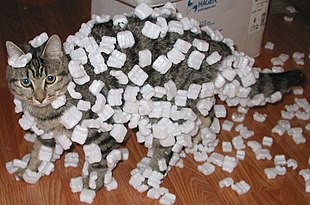
Evidence of an electric field: styrofoam peanuts clinging to a cat's fur due to static electricity. The triboelectric effect causes an electrostatic charge to build up on the fur due to the cat's motions. The electric field of the charge causes polarization of the molecules of the styrofoam due to electrostatic induction, resulting in a slight attraction of the light plastic pieces to the charged fur. This effect is also the cause of static cling in clothes.

The Coulomb force on a charge of magnitude qdisplaystyle q at any point in space is equal to the product of the charge and the electric field at that point

F=qEdisplaystyle boldsymbol F=qboldsymbol E

The units of the electric field in the SI system are newtons per coulomb (N/C), or volts per meter (V/m); in terms of the SI base units they are kg⋅m⋅s⁻³⋅A⁻¹

The electric field due to a continuous distribution of charge ρ(x)displaystyle rho (boldsymbol x) in space (where ρdisplaystyle rho is the charge density in coulombs per cubic meter) can be calculated by considering the charge ρ(x′)dVdisplaystyle rho (boldsymbol x')dV in each small volume of space dVdisplaystyle dV at point x′displaystyle boldsymbol x' as a point charge, and calculating its electric field dE(x)displaystyle dboldsymbol E(boldsymbol x) at point xdisplaystyle boldsymbol x

dE(x)=14πε0ρ(x′)dV(x′−x)2r^′displaystyle dboldsymbol E(boldsymbol x)=1 over 4pi varepsilon _0rho (boldsymbol x')dV over (boldsymbol x'-x)^2boldsymbol hat r'

where r^′displaystyle boldsymbol hat r' is the unit vector pointing from x′displaystyle boldsymbol x' to xdisplaystyle boldsymbol x, then adding up the contributions from all the increments of volume by integrating over the volume of the charge distribution Vdisplaystyle V

E(x)=14πε0∭Vρ(x′)dV(x′−x)2r^′displaystyle boldsymbol E(boldsymbol x)=1 over 4pi varepsilon _0iiint limits _V,rho (boldsymbol x')dV over (boldsymbol x'-x)^2boldsymbol hat r'

Sources

Causes and description

Electric fields are caused by electric charges, described by Gauss's law,^[7] or varying magnetic fields, described by Faraday's law of induction.^[8] Together, these laws are enough to define the behavior of the electric field as a function of charge repartition and magnetic field. However, since the magnetic field is described as a function of electric field, the equations of both fields are coupled and together form Maxwell's equations that describe both fields as a function of charges and currents.

In the special case of a steady state (stationary charges and currents), the Maxwell-Faraday inductive effect disappears. The resulting two equations (Gauss's law ∇⋅E=ρε0displaystyle nabla cdot mathbf E =frac rho varepsilon _0 and Faraday's law with no induction term ∇×E=0displaystyle nabla times mathbf E =0), taken together, are equivalent to Coulomb's law, written as E(r)=14πε0∫ρ(r′)r−r′|r−r′|3d3r′displaystyle boldsymbol E(boldsymbol r)=1 over 4pi varepsilon _0int rho (boldsymbol r')boldsymbol r-boldsymbol r' over d^3r' for a charge density
ρ(r)displaystyle mathbf rho (mathbf r ) (rdisplaystyle mathbf r denotes the position in space).^[9] Notice that ε0displaystyle varepsilon _0, the permitivity of vacuum, must be substituted if charges are considered in non-empty media.

Continuous vs. discrete charge representation

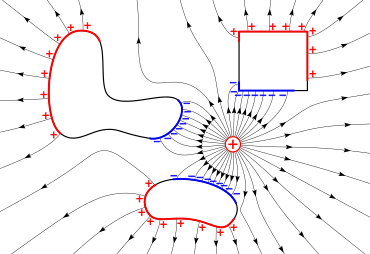
The electric field (lines with arrows) of a charge (+) induces surface charges (red and blue areas) on metal objects due to electrostatic induction.

The equations of electromagnetism are best described in a continuous description. However, charges are sometimes best described as discrete points; for example, some models may describe electrons as point sources where charge density is infinite on an infinitesimal section of space.

A charge qdisplaystyle q located at r0displaystyle mathbf r_0 can be described mathematically as a charge density ρ(r)=qδ(r−r0)displaystyle rho (mathbf r )=qdelta (mathbf r-r_0 ), where the Dirac delta function (in three dimensions) is used. Conversely, a charge distribution can be approximated by many small point charges.

Superposition principle

Electric fields satisfy the superposition principle, because Maxwell's equations are linear. As a result, if E1displaystyle mathbf E _1 and E2displaystyle mathbf E _2 are the electric fields resulting from distribution of charges ρ1displaystyle rho _1 and ρ2displaystyle rho _2, a distribution of charges ρ1+ρ2displaystyle rho _1+rho _2 will create an electric field E1+E2displaystyle mathbf E _1+mathbf E _2; for instance, Coulomb's law is linear in charge density as well.

This principle is useful to calculate the field created by multiple point charges. If charges q1,q2,...,qndisplaystyle q_1,q_2,...,q_n are stationary in space at r1,r2,...rndisplaystyle mathbf r _1,mathbf r _2,...mathbf r _n, in the absence of currents, the superposition principle proves that the resulting field is the sum of fields generated by each particle as described by Coulomb's law:

E(r)=∑i=1NEi(r)=14πε0∑i=1Nqir−ri|r−ri|3displaystyle mathbf E (mathbf r )=sum _i=1^Nmathbf E _i(mathbf r )=frac 14pi varepsilon _0sum _i=1^Nq_ifrac mathbf r -mathbf r _i^3

Electrostatic fields

Illustration of the electric field surrounding a positive (red) and a negative (blue) charge

Play media

Experiment illustrating electric field lines. An electrode connected to an electrostatic induction machine is placed in an oil-filled container. Considering that oil is a dielectric medium, when there is current through the electrode, the particles arrange themselves so as to show the force lines of the electric field.

Electrostatic fields are electric fields which do not change with time, which happens when charges and currents are stationary. In that case, Coulomb's law fully describes the field.^[10]

Electric potential

If a system is static, such that magnetic fields are not time-varying, then by Faraday's law, the electric field is curl-free. In this case, one can define an electric potential, that is, a function Φdisplaystyle Phi such that E=−∇Φdisplaystyle mathbf E =-nabla Phi .^[11]
This is analogous to the gravitational potential.

Parallels between electrostatic and gravitational fields

Coulomb's law, which describes the interaction of electric charges:

F=q(Q4πε0r^|r|2)=qEdisplaystyle mathbf F =qleft(frac Q4pi varepsilon _0frac mathbf hat r ^2right)=qmathbf E "/>

is similar to Newton's law of universal gravitation:

F=m(−GMr^|r|2)=mgdisplaystyle mathbf F =mleft(-GMfrac mathbf hat r ^2right)=mmathbf g "/>

(where r^=r|r|displaystyle mathbf hat r =mathbf frac r ).

This suggests similarities between the electric field E and the gravitational field g, or their associated potentials. Mass is sometimes called "gravitational charge" because of that similarity.^{[citation needed]}

Electrostatic and gravitational forces both are central, conservative and obey an inverse-square law.

Uniform fields

A uniform field is one in which the electric field is constant at every point. It can be approximated by placing two conducting plates parallel to each other and maintaining a voltage (potential difference) between them; it is only an approximation because of boundary effects (near the edge of the planes, electric field is distorted because the plane does not continue). Assuming infinite planes, the magnitude of the electric field E is:

E=−Δϕddisplaystyle E=-frac Delta phi d

where Δϕ is the potential difference between the plates and d is the distance separating the plates. The negative sign arises as positive charges repel, so a positive charge will experience a force away from the positively charged plate, in the opposite direction to that in which the voltage increases. In micro- and nano-applications, for instance in relation to semiconductors, a typical magnitude of an electric field is in the order of 7006100000000000000♠10⁶ V⋅m⁻¹, achieved by applying a voltage of the order of 1 volt between conductors spaced 1 µm apart.

Electrodynamic fields

Electrodynamic fields are electric fields which do change with time, for instance when charges are in motion.

The electric field cannot be described independently of the magnetic field in that case. If A is the magnetic vector potential, defined so that B=∇×Adisplaystyle mathbf B =nabla times mathbf A , one can still define an electric potential Φdisplaystyle Phi such that:

E=−∇Φ−∂A∂tdisplaystyle mathbf E =-nabla Phi -frac partial mathbf A partial t

One can recover Faraday's law of induction by taking the curl of that equation

^[12]

∇×E=−∂(∇×A)∂t=−∂B∂tdisplaystyle nabla times mathbf E =-frac partial (nabla times mathbf A )partial t=-frac partial mathbf B partial t

which justifies, a posteriori, the previous form for E.

Energy in the electric field

The total energy per unit volume stored by the electromagnetic field is^[13]

uEM=ε2|E|2+12μ|B|2mathbf B

where ε is the permittivity of the medium in which the field exists, μdisplaystyle mu its magnetic permeability, and E and B are the electric and magnetic field vectors.

As E and B fields are coupled, it would be misleading to split this expression into "electric" and "magnetic" contributions. However, in the steady-state case, the fields are no longer coupled (see Maxwell's equations). It makes sense in that case to compute the electrostatic energy per unit volume:

uES=12ε|E|2,^2,,

The total energy U stored in the electric field in a given volume V is therefore

UES=12ε∫V|E|2dV,^2,mathrm d V,,

Further extensions

Definitive equation of vector fields

In the presence of matter, it is helpful to extend the notion of the electric field into three vector fields:^[14]

D=ε0E+Pdisplaystyle mathbf D =varepsilon _0mathbf E +mathbf P !

where P is the electric polarization – the volume density of electric dipole moments, and D is the electric displacement field. Since E and P are defined separately, this equation can be used to define D. The physical interpretation of D is not as clear as E (effectively the field applied to the material) or P (induced field due to the dipoles in the material), but still serves as a convenient mathematical simplification, since Maxwell's equations can be simplified in terms of free charges and currents.

Constitutive relation

The E and D fields are related by the permittivity of the material, ε.^[15][14]

For linear, homogeneous, isotropic materials E and D are proportional and constant throughout the region, there is no position dependence: For inhomogeneous materials, there is a position dependence throughout the material:

D(r)=εE(r)displaystyle mathbf D(r) =varepsilon mathbf E(r)

For anisotropic materials the E and D fields are not parallel, and so E and D are related by the permittivity tensor (a 2nd order tensor field), in component form:

Di=εijEjdisplaystyle D_i=varepsilon _ijE_j

For non-linear media, E and D are not proportional. Materials can have varying extents of linearity, homogeneity and isotropy.

See also

• Classical electromagnetism


• Field strength


• 
  Signal strength in telecommunications


• Magnetism


• Teltron tube


• 
  Teledeltos, a conductive paper that may be used as a simple analog computer for modelling fields

References

• 
  Purcell, Edward; Morin, David (2010). ELECTRICITY AND MAGNETISM (3rd ed.). Cambridge University Press, New York. ISBN 978-1-107-01402-2.CS1 maint: Multiple names: authors list (link)
  


• 
  Browne, Michael (2011). PHYSICS FOR ENGINEERING AND SCIENCE (2nd ed.). McGraw-Hill, Schaum, New York. ISBN 978-0-07-161399-6.
  

External links

Wikimedia Commons has media related to Electric field.

This article's use of external links may not follow Wikipedia's policies or guidelines. Please improve this article by removing excessive or inappropriate external links, and converting useful links where appropriate into footnote references. (January 2017) (Learn how and when to remove this template message)

• 
  Electric field in "Electricity and Magnetism", R Nave – Hyperphysics, Georgia State University
  


• 
  'Gauss's Law' – Chapter 24 of Frank Wolfs's lectures at University of Rochester
  


• 
  'The Electric Field' – Chapter 23 of Frank Wolfs's lectures at University of Rochester
  


• 
  MovingCharge.html – An applet that shows the electric field of a moving point charge


• 
  Fields – a chapter from an online textbook


• 
  Learning by Simulations Interactive simulation of an electric field of up to four point charges


• 
  Interactive Flash simulation picturing the electric field of user-defined or preselected sets of point charges by field vectors, field lines, or equipotential lines. Author: David Chappell

References

^ Purcell and Morin, Harvard University. (2013). Electricity and Magnetism, 820pages (3rd ed.). Cambridge University Press, New York. ISBN 978-1-107-01402-2..mw-parser-output cite.citationfont-style:inherit.mw-parser-output qquotes:"""""""'""'".mw-parser-output code.cs1-codecolor:inherit;background:inherit;border:inherit;padding:inherit.mw-parser-output .cs1-lock-free abackground:url("//upload.wikimedia.org/wikipedia/commons/thumb/6/65/Lock-green.svg/9px-Lock-green.svg.png")no-repeat;background-position:right .1em center.mw-parser-output .cs1-lock-limited a,.mw-parser-output .cs1-lock-registration abackground:url("//upload.wikimedia.org/wikipedia/commons/thumb/d/d6/Lock-gray-alt-2.svg/9px-Lock-gray-alt-2.svg.png")no-repeat;background-position:right .1em center.mw-parser-output .cs1-lock-subscription abackground:url("//upload.wikimedia.org/wikipedia/commons/thumb/a/aa/Lock-red-alt-2.svg/9px-Lock-red-alt-2.svg.png")no-repeat;background-position:right .1em center.mw-parser-output .cs1-subscription,.mw-parser-output .cs1-registrationcolor:#555.mw-parser-output .cs1-subscription span,.mw-parser-output .cs1-registration spanborder-bottom:1px dotted;cursor:help.mw-parser-output .cs1-hidden-errordisplay:none;font-size:100%.mw-parser-output .cs1-visible-errorfont-size:100%.mw-parser-output .cs1-subscription,.mw-parser-output .cs1-registration,.mw-parser-output .cs1-formatfont-size:95%.mw-parser-output .cs1-kern-left,.mw-parser-output .cs1-kern-wl-leftpadding-left:0.2em.mw-parser-output .cs1-kern-right,.mw-parser-output .cs1-kern-wl-rightpadding-right:0.2em
^ Browne, p 225: "... around every charge there is an aura that fills all space. This aura is the electric field due to the charge. The electric field is a vector field... and has a magnitude and direction."
^ Richard Feynman (1970). The Feynman Lectures on Physics Vol II. Addison Wesley Longman. ISBN 978-0-201-02115-8.
^ ab Purcell, Edward (2011). Electricity and Magnetism, 2nd Ed. Cambridge University Press. pp. 8–9, 15–16. ISBN 11395035538 Check|isbn=value: length (help).
^ abc Serway, Raymond A.; Vuille, Chris (2014). College Physics, 10th Ed. Cengage Learning. pp. 532–533. ISBN 1305142829.
^ Purcell (2011) Electricity and Magnetism, 2nd Ed., p. 20-21
^ Purcell, p 25: "Gauss's Law: the flux of the electric field E through any closed surface... equals 1/e times the total charge enclosed by the surface."
^ Purcell, p 356: "Faraday's Law of Induction."
^ Purcell, p7: "... the interaction between electric charges at rest is described by Coulomb's Law: two stationary electric charges repel or attract each other with a force proportional to the product of the magnitude of the charges and inversely proportional to the square of the distance between them.
^ Purcell, p5-7.
^ gwrowe (8 October 2011). "Curl & Potential in Electrostatics". physicspages.com. Retrieved 21 January 2017.
^ Huray, Paul G. (2009). Maxwell's Equations. Wiley-IEEE. p. 205. ISBN 0-470-54276-4.
^ Introduction to Electrodynamics (3rd Edition), D.J. Griffiths, Pearson Education, Dorling Kindersley, 2007,
ISBN 81-7758-293-3
^ ab Electromagnetism (2nd Edition), I.S. Grant, W.R. Phillips, Manchester Physics, John Wiley & Sons, 2008,
ISBN 978-0-471-92712-9
^ Electricity and Modern Physics (2nd Edition), G.A.G. Bennet, Edward Arnold (UK), 1974,
ISBN 0-7131-2459-8